Galaxy classification using the random forest algorithm

If you’ve read any current research on the morphological classification of galaxies, you probably know that CNNs (convoluted neural networks) are one of the most popular choices of classifiers used. In comparison, many older articles use algorithms like Random Forest and XGBoost (eXtreme Gradient Boosting) which are based on more traditional classifiers like decision trees. In this article, I’ll revisit the random forest approach, and compare it to a neural network in the next part to find out which choice is better!

The morphological classification of galaxies

Okay, short astronomy lesson first. In the 1920’s, Edwin Hubble created a system commonly called the ‘Hubble tuning fork diagram’, to classify galaxies based on their appearances while studying their evolution. This system is still very commonly used today (although now considered a bit of an oversimplification), and is divided into two distinct parts: elliptical, and spiral galaxies. The ellipticals are further divided into 7 subcategories, with E0 being the least elliptical (a.k.a the roundest), and E7 being the most elliptical. Spirals on the other hand, are broken down further into ‘S’ (normal spirals) and ‘SB’ (barred spirals), based on how the spiral arms project from the center of the galaxy. Both of these divisions are then given suffixes from a-c, with ‘a’ being the tightest wound spiral and ‘c’ being the loosest. There is also a special type of galaxies placed right where the prongs of the ‘tuning fork’ meet its stem, S0 or lenticular galaxies, which are considered transitional galaxies exhibiting features of both spirals and ellipticals. One thing that this diagram doesn’t account for however, is the existence of irregular galaxies, which are neither elliptical nor spiral in shape, usually formed as a result of collisions/interactions amongst galaxies.

But why is any of this important? Well, even though Hubble’s original concept of galaxy evolution wasn’t completely accurate, the appearance of a galaxy can actually tell us a lot about what goes on inside. The arms of spiral galaxies are sites of star formation, containing large amounts of hot gas and dust that give birth to bright, hot, and young stars (most type O and B on the HR diagram). Elliptical galaxies on the other hand are referred to as ‘red and dead’ galaxies, since they contain less gas and dust, and are populated by older, redder stars with long lifespans.

CNNs and Random Forests

For the purpose of this model, I’m using labelled images from the publicly available Galaxy Zoo dataset (https://www.zooniverse.org/projects/zookeeper/galaxy-zoo/) on Zooniverse.

As I mentioned earlier, two of the most common approaches to classification are CNNs and Random Forest. The simplest way I can explain how CNNs work is by using convolution layers that detect features like edges and lines to create feature maps for different filters (more about this in part 2). While this method is extremely accurate, the problem with neural networks is that they sort of act like a black box. What I mean by this is that the output of such classifiers is not interpretable, so you won’t get much insight as to why a galaxy is classified the way it is. Keep in mind that this holds true mostly for vanilla CNNs, and that new techniques detecting which regions most influence the classifier’s decision have been developed.

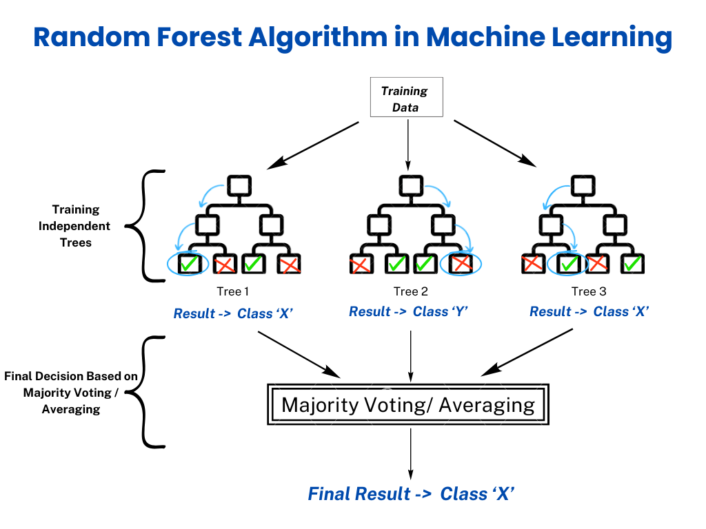
This brings me to Random Forests, which is the method I’m going to use to classify the galaxy zoo dataset in this article. Like a regular forest is made up of regular trees, in machine learning, a random forest is made up of multiple decision trees. A decision tree is basically a flowchart-style model that starts at the ‘root node’, which is the main question derived from the features of the dataset. From then onwards, it asks a series of yes/no questions, splitting the data into subsets based on specific features, reaching a conclusion (leaf node) when there are no more useful questions to be asked.

Decision trees have their own share of problems, which include overfitting, where the trees get so deep that they memorize the training data instead of underlying patterns, and instability. In an attempt to reduce this, we use random forests instead of depending on the output of one, singular tree. There are roughly three main parts to the working of a random forest: bootstrapping, random feature selection (feature bagging), and aggregation. You may have heard this type of random forest, where the decision trees work parallel to each other producing independent results, be sometimes referred to as Bagging (bootstrapping + aggregation).

1. Bootstrapping - The selection of random data values within the original dataset for each decision tree.
2. Random feature selection - The selection of a random subset of the total features to train each individual decision tree on. This helps decorrelate them, reducing the chances of getting overfitted results.
3. Aggregation - Averaging (in case of regression), or taking a majority vote (in case of classification) from each decision tree to reach a conclusion.

Choosing defining features for galaxies

So now we know that we need to train the random forest on some features of the galaxies, but what features exactly do we use, given our dataset consists of images?
Well, for each image in the training and testing data, I computed a small set of non‑parametric structural features that define how the galaxy’s light is distributed. To do this, I treated each image as a 2D light distribution, and found the flux-weighted centroid (the center that lies near the brightness peak), which I then used to find the radial distance of each pixel. This is because galaxies are roughly centrally concentrated, so defining everything with respect to the center lets us build accurate radial profiles and flux fractions.

Radial profiles are the radii containing some portion of the total light of the galaxy. I use three common radial profiles as features to train my random forest: R20, R50, and R80, the radii at which the cumulative flux reaches 20%, 50%, and 80% of itself respectively. Since elliptical galaxies have a lot of their light packed into a small radius, we expect them to have a smaller R20 and R50, whereas other, more spread out galaxies tend to have higher values for these features.

Using these radial profiles, we can calculate concentration indices, which quantify how centrally concentrated the light is. As my fourth and fifth features, I use the 50/20 and 80/20 concentration indices, which can be calculated as R50/R20 and R80/R20 respectively. As we outlined earlier, elliptical galaxies tend to be more centrally concentrated, and thus have higher concentration indices as compared to other featured galaxies such as spirals and irregulars.

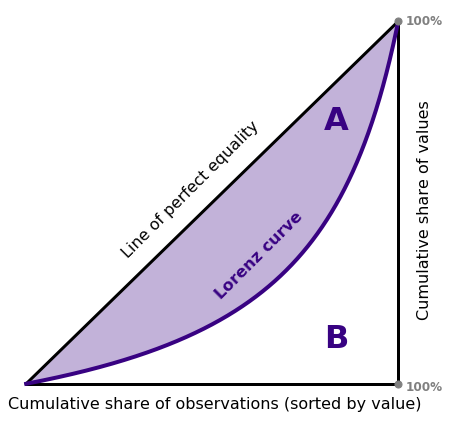
For my next feature, I calculated the Gini coefficient, a term you may have heard of in Economics used to calculate income inequality. In our case, the Gini Coefficient or G is value from 0-1 used to measure how unequally the total light is distributed among pixels. If a few pixels are very bright and most are faint, the distribution is highly unequal (high G). If brightness is uniform, Gini is low.

The final feature I calculated was M20, the second moment of the brightest 20% of pixels. The value of M20 describes how spatially extended the brightest regions are. If the brightest 20% of light is near the center like in ellipticals, you get a low M20; if it is more off‑center, M20 becomes larger.

Extracting features computationally

To start with the model, we’ll first need to import and filter our dataset. As mentioned before, I’m using data from the galaxy zoo project, which contains 120,000 classified images from the Hubble Space Telescope. More specifically, I’ll use the 'smooth-or-featured-gz2_smooth' label column within the dataset to filter galaxies that exhibit smooth, elliptical shapes vs. featured galaxies that have arms, bars or irregularities based citizens' votes in the Galaxy Zoo project. A vote>0.5 means the galaxy is smooth, and <0.5 means its featured. You can import the training dataset into your code as follows:

from galaxy_datasets import gz2
import numpy as np
import pandas as pd
from PIL import Image

catalog, label_cols = gz2(
    root="data",
    train=True,
    download=True
)

But, before we can actually use these images, we need to clean them up a bit. I wrote a tiny function that does this by converting the images to grayscale and roughly subtracting their background (~5th percentile).

import os
def load_image_gray(path):
    im = Image.open(path).convert("L")        #grayscale
    arr = np.array(im, dtype=np.float32)
    arr -= np.percentile(arr, 5)             #rough background subtraction
    arr[arr < 0] = 0
    return arr

Now, we can start on a function to calculate the 7 features outlined in the part above from each image.

def compute_features(img):
    yy, xx = np.indices(img.shape)
    #computing a flux-weighted centroid
    total_flux = img.sum()
    #sub pixel center that lands near the brightness peak
    x_centroid = (xx * img).sum() / total_flux 
    y_centroid = (yy * img).sum() / total_flux
    r = np.sqrt((xx - x_centroid)**2 + (yy - y_centroid)**2)
    r_max = r.max()
    bins = np.linspace(0, r_max, num=20) #20 bins for radius
    r_flat = r.ravel()
    img_flat = img.ravel()
    which_bin = np.digitize(r_flat, bins) - 1
    mean_flux = np.zeros(len(bins))
    r_mid = []
    for i in range(len(bins)):
        mean_flux[i] = img_flat[which_bin == i].mean()
        r_mid.append(0.5 * (bins[i] + bins[i-1]) if i > 0 else bins[0] / 2)

    cumulative_flux = np.cumsum(mean_flux)
    total_cumulative_flux = cumulative_flux[-1]

This piece of code basically adds up the brightness for each pixel in the image and stores it in total_flux. Then, treating the image as a 2d distribution, it calculates the centroid, which is where the brightness peaks, and uses it to calculate the radial distances for each pixel. It then creates 20 concentric annuli (area betw. 2 concentric circles) from the center to the max radius, taking the mean flux of all pixels in that annulus to calculate approximate azimuthally averaged radial profiles as shown below:

    R20 = r_mid[np.searchsorted(cumulative_flux, 0.2 * total_cumulative_flux)]
    R50 = r_mid[np.searchsorted(cumulative_flux, 0.5 * total_cumulative_flux)]
    R80 = r_mid[np.searchsorted(cumulative_flux, 0.8 * total_cumulative_flux)]
    C_80_20 = R80 / R20 if R20 !=0 else 0 
    C_50_20 = R50 / R20 if R20 !=0 else 0
    f = np.sort(img.ravel().copy())
    f[f < 0] = 0

The radial profile calculations use Numpy’s searchsorted function to find the bins where the cumulative flux first reaches 20%, 50% and 80% of itself respectively, taking their midpoints as R20, R50 and R80.
Following this, it finds the concentration indices by calculating ratios of the radial profiles.

We can now move on to calculating the Gini coefficient and M20.

    # Gini coefficient
    #Gini coeff = inequality in brightness across the pixels 
    n = f.size
    mean_f = f.mean()
    i = np.arange(1, n+1)  # 1..n
    G = ( (2*i - n - 1) * f ).sum() / (mean_f * n * (n-1) + 1e-8)

    xx_f = xx.ravel()
    yy_f = yy.ravel()
    r2 = (xx_f - x_centroid)**2 + (yy_f - y_centroid)**2
    M_i = f * r2
    idx_desc = np.argsort(f)[::-1]
    f_desc = f[idx_desc]
    M_desc = M_i[idx_desc]
    cum_flux_desc = np.cumsum(f_desc)
    total_flux = f_desc.sum()
    k = np.searchsorted(cum_flux_desc, 0.2 * total_flux) + 1
    M20_sum = M_desc[:k].sum()
    positive = f > 0
    f = f[positive]; xx_f = xx_f[positive]; yy_f = yy_f[positive]
    r2 = (xx_f - x_centroid)**2 + (yy_f - y_centroid)**2

    M_i = f * r2
    M_tot = M_i.sum()

    idx_desc = np.argsort(f)[::-1]
    f_desc = f[idx_desc]
    M_desc = M_i[idx_desc]

    cum_flux = np.cumsum(f_desc)
    k = np.searchsorted(cum_flux, 0.2 * cum_flux[-1]) + 1
    M20_sum = M_desc[:k].sum()

    M20 = np.log10(M20_sum / (M_tot + 1e-8))
    features = np.array([
    R20, R50, R80,
    C_80_20, C_50_20,
    G, M20
    ], dtype=np.float32)

    return np.array(features, dtype=np.float32)

First, I flatten all the pixel values into a one‑dimensional list and plug them into the standard Gini formula (attached below), which gives me the Gini coefficient G. Pixels that are all about the same brightness give a low Gini while a few very bright pixels and lots of faint ones give a high Gini.

For M20, I combine each pixel’s brightness with its distance from the galaxy’s center (radial distance). I flatten the x–y pixel coordinates, compute the distance of every pixel from the centroid, and then multiply that distance squared by the pixel’s brightness. That gives a “moment” for each pixel: bright pixels far from the center contribute a lot, faint pixels near the center contribute little. I then sort pixels from brightest to faintest and start adding up their moments until I’ve included just the brightest 20% of the total light. The sum of those moments, divided by the total moment of the whole galaxy and put through a logarithm, gives us M20. Finally, I return everything-radii, concentration, Gini, and M20-as a small feature vector which my random forest model can then use to learn the difference between smooth and featured galaxies.

You can then loop over the Galaxy Zoo training dataset and run this function for each image, storing the results in an array called X_train, and the corresponding labels (1 if label>0.5, 0 otherwise) in y_train. However, be aware that it takes over 1000 minutes to complete… I suggest saving the features of every 100-500 images you process into a CSV file as you go. Also, wrap the entire code in a try-except block so that a small error doesn't ruin hours of computation (I learned this the hard way).

Once you do everything above successfully, you’ll be ready to move onto downloading test data! You can do this the same way we did at the top of this section, just by changing the parameter train to false :

catalog_test, label_cols = gz2(
    root="data",
    train=False,
    download=False 
)

You can then run the function compute_features for every image in this dataset too, storing the results in X_test and y_test as done earlier.

Building the random forest

Finally, we can start with the most awaited section of this article, training and evaluating our random forest model!

from sklearn.ensemble import RandomForestClassifier
import matplotlib.pyplot as plt
from sklearn.metrics import confusion_matrix
import numpy as np
import pandas as pd

model = RandomForestClassifier(n_estimators=100)
cols = ['R20','R50','R80','C_80_20','C_50_20','Gini','M20']
X_train =  pd.read_csv("brightness_features_train.csv", usecols=cols).values
y_train = pd.read_csv('brightness_features_train.csv', usecols=['label']).values
model.fit(X_train, y_train)
X_test = pd.read_csv("brightness_features_test2.csv", usecols=cols).values
y_test = pd.read_csv('brightness_features_test2.csv', usecols=['label']).values
model.score(X_test, y_test)
y_predict = model.predict(X_test)
cm = confusion_matrix(y_test, y_predict)
plt.imshow(cm, cmap='Blues')
plt.colorbar()
plt.xlabel('Predicted labels')
plt.ylabel('True labels')
plt.xticks([0, 1], ['Featured', 'Smooth'])
plt.yticks([0, 1], ['Featured', 'Smooth'])
plt.title('Confusion Matrix')
plt.show()

Here, I use Scikitlearn’s RandomForestClassifier function to create a model with 100 decision trees (n_estimators), and feed in the features I computed for the training dataset, plus a binary label (label = 0 for featured, 1 for smooth). Then I point the model at the test set, ask it to predict smooth vs featured, and build a confusion matrix: a 2×2 grid that shows, for each true class, how many times the model predicted featured or smooth.

This approach seems reasonable, but in practice, it fails for two reasons. First, the labels are hugely skewed: only a few percent of galaxies in Galaxy Zoo are tagged as “featured” by the vote fraction cut I used, while almost everything else is “smooth.” You can actually find the exact number of featured to smooth galaxies by running the following line:

print("Train:", np.bincount(y_train.ravel().astype(int)))

This returns ‘Train: [ 3116 126644]’, which means that in the training dataset, there are only 3,116 featured galaxies for 126,644 smooth ones, or 2% featured for 98% smooth.

That means a dumb model that simply classifies every single galaxy as “smooth”, already hits around 98% accuracy. Second, the seven global brightness features I chose don’t cleanly separate these two classes at survey quality; many featured galaxies have very similar light profiles and Gini/M20 values to smooth ones. Put those together, and the random forest learns that the safest move is to call almost everything smooth. The confusion matrix ends up with one giant block in the “true smooth / predicted smooth” cell, almost nothing in the “true featured / predicted featured” cell, and accuracy that looks great but is scientifically useless.

One step I took to fix this, was to weigh the featured galaxies as much as the smooth ones, by creating a new training dataset consisting of a 50-50 ratio of featured to smooth galaxies. This resulted in a confusion matrix looking something like this:

This means that the model just predicted more false ‘featured’s, reducing the accuracy of the model to around 55%, which clearly does not fix the problem at all.

Conclusion

So, as we just saw, the random forest approach almost completely failed. It couldn’t reliably pick out featured galaxies from the very skewed Galaxy Zoo data, even when the training set was rebalanced. It either defaulted to calling almost everything smooth or produced lots of false featured flags, which tells us these seven features aren’t enough information for this type of classification. In the next part, we’ll look at how much better CNNs do when they can look directly at the full galaxy images, and then talk about why their decisions differ from the simpler model.

Thank you, and happy holidays!