Simulating the cosmological N-body problem (new)
...and why astrophysicists are yet to solve it
An aspiring developer
I was never really one to listen to podcasts (reading is simply superior), but I recently got into the habit of listening to Neil DeGrasse Tyson’s ‘StarTalk’ on my 30-minute bus ride to school, and it’s become my favorite part of the day. One particular episode that caught my attention was his discussion on the unsolvable 3-body problem. He describes it as "three objects of roughly the same mass trying to maintain a stable orbit" and notes that it is mathematically chaotic to solve. Building on this topic, in this article, I'll explore the n-body problem (a more generalized version of the 3-body problem) and attempt to simulate it computationally using Python!
What is the N-body Problem?
While we have equations that can completely predict the interactions of 2 gravitational masses (thank you, Newton), the complexity of systems with 3 or more bodies makes their movement impossible to predict. This is what astrophysicists label as the n-body problem. The issue with writing down a general formula to describe the motion of three or more gravitating objects is that we have more unknowns than equations describing them, a.k.a, there are way too many variables to deal with! But what does it mean for these systems to be chaotic? Mathematically, the word ‘chaotic’ is used to refer to a system that is deterministic (non-random), but highly sensitive to its initial conditions (commonly referred to as the butterfly effect). We see this in the n-body problem, where every configuration of these bodies has a large range of potential outcomes that are influenced by the tiniest change in velocity or position.
Forces and motion
Now that we know what the problem is, we can try to write it mathematically.

Here, we have three masses M1, M2 and Mi along with their distance vectors. We can use the equation for the force of attraction between 2 bodies i and j using the Newtonian equation of gravity :

Here, rj - ri gives us the position vector from mass i to mass j, along which the force of attraction acts.
The reason the force is negative, is because of the inverse relationship of the position and force of attraction vectors. While the position vector Rj-Ri points AWAY from mass i, the force of attraction points TOWARDS IT.
Note : j ≠ i here, because it would make the denominator 0 (also, how would you calculate the attraction from a body to… itself?)
In an n-body simulation, you don’t have just 2 bodies, you have an n number of bodies. This means that you have to sum up all the forces acting on the body , as such :

The problem with this equation is that it does not account for cases when 2 more more bodies are extremely close, which makes the denominator ~ 0 resulting in singularity. As a solution, I softened the force using the Plummer potential, by adding a tiny constant ε (epsilon) as such:

This value of ε can be calculated by the following formula, where R is the virial radius, and n is the number of bodies in the simulation:

Now, to implement this in our code we can write a function as shown below to calculate the forces on each individual star:
def calc_forces():
    for star in stars:
        star.F = vector(0, 0, 0)

    for i in range(len(stars)):
        for j in range(len(stars)):
            if i != j:
                rji = stars[j].pos - stars[i].pos
                dist = mag(rji)
                stars[i].F += G * stars[i].m * stars[j].m * norm(rji) math.pow((dist**2 + e**2),3/2)
                stars[j].F -= G * stars[i].m * stars[j].m * norm(rji) / math.pow((dist**2 + e**2),3/2)
The first loop goes over every star in both lists, and calculates the force of attraction they exert on each other using the formula shown earlier. Notice that we use VPython’s norm() function to normalize the position vector, which removes the extra magnitude from the denominator of the equation. For each individual star (star[i]), I sum up the forces on it from the other stars (star[j]). I then add this value to star[i] and subtract it from star[j] (according to Newton's third law, each action has an equal and opposite reaction)
Assigning Initial Positions and Velocities Following a Plummer Sphere
To make the simulation more realistic, I generated the initial positions and velocities of the N stars such that they follow the Plummer sphere model’s mass and potential profiles. The total mass contained within a sphere of radius r is given by the following formula:

Every star can contain a fraction M(r)/M of the total mass M within its radial position. Considering the mass of the entire system/cluster as 1, we can then generated N random numbers from 0-1 to represent the M(r). The mass fraction could be anything between 0 and 1. It will be 0 if the particle is placed exactly in the center, and it will approach 1 as the particle is placed further away, reaching 1 at infinity. To solve for r, we can rewrite the equation as such, where Xi is the i-th random mass :

Now that we have our radii, we can use spherical polar coordinates (r,θ,φ) to get the actual positions of the stars as a 3d vector.

x = r sin(θ) cos(φ)
y = r sin(θ) sin(φ)
z = r cos(θ)
φ (phi), is the azimuthal angle that measures the horizontal rotation and lies between 0 and 2𝜋.
θ (theta), is the polar angle that measures vertical tilt (from the z axis in this case) and is calculated such that cos θ lies between -1 and 1.
r is the radius we calculated above.
Again, we can calculate uniformly random numbers within these ranges for θ and φ.
Let’s now begin to simulate the n-body problem for an n number of stars using VPython. Like most libraries, you can install VPython using pip and import it using from vpython import *
G = 1
M = 1
R = 1
N = input("Number of bodies to simulate: ")
stars = []
To start, I’m defining all the constants as 1 to avoid dealing with really small numbers. Also, I get the number of stars to simulate movement for from the user and store it in the constant N. stars[], is an empty list we will use to store the stars we create later on in our program.
We can then start building our ‘Star’ class, which will act as a template for every star we create.
class Star:
    def __init__(self, pos, v, M):
        self.pos = pos
        self.m = M
        self.v = v
        self.p = self.m * self.v
        self.F = vector(0, 0, 0)
        self.a = self.F/self.m
        self.sphere = sphere(pos=self.pos, radius=R / 30, make_trail=True, retain=100, color = vector(random(), random(), random()))
Every star created using the Star class will have a position (passed in as a parameter), a radius, a velocity, a mass, momentum, acceleration and force (initialized to a vector with magnitude 0). We then draw the star onto the screen by creating a sphere with the given position, radius, and a random color.
We can now use the method discussed above to generate random positions for each of the stars as such:
def plummer_sphere(a=1.0):
    Xi = np.random.uniform(0, 1)

    r = a / np.sqrt(Xi**(-2/3) - 1)

    theta = np.arccos(np.random.uniform(-1, 1)) #polar angle
    phi = np.random.uniform(0, 2 * np.pi) #azimuthal angle

    #our actual coordinates
    x = r * np.sin(theta) * np.cos(phi)
    y = r * np.sin(theta) * np.sin(phi)
    z = r * np.cos(theta)
But, what about the velocities? Well, the maximum velocity at any given coordinate on the plummer sphere is the escape velocity, given by the formula -
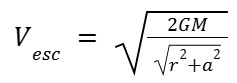
Therefore the initial velocity of every star in the simulation must be between 0 and the escape velocity (Vesc). In order to get the velocity, we need to know its distribution function, which in this case is given by:
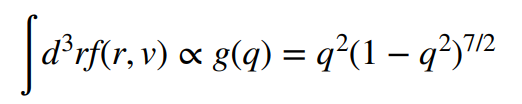
Here, q is the ratio between the stars' individual velocities and the escape velocity (q = V/Vesc). Where q ∈ [0,1] and g(q) ∈ [0,0.1]. To find a fit to this PDF, there are generally two directions you can take - rejection sampling, or the Newton root-finding method. I will be using the former. To implement Von Neumann rejection sampling, I sample 2 uniformly random numbers x and y in the range [0,1]. For each pair, if 0.01*y < g(x), I accept q = x.
Since velocities are isotropic (same magnitude in all directions) I use the same method for the positions to assign random directions to the velocities.
To implement this, I extend my plummer_sphere() function as such:
 v_esc = np.sqrt(2 * G * M / np.sqrt(r**2 + a**2))
 v_mag = 0
 q = 0.0

while True:
    q = np.random.uniform(0, 1)

    g_q = 0.1 * np.random.uniform(0, 1)
    if g_q < (q**2 * (1 - q**2)**3.5):
        v_mag = q * v_esc
        break

#random direction for velocity vector just like the coordiantes
v_theta = np.arccos(np.random.uniform(-1, 1))
v_phi = np.random.uniform(0, 2 * np.pi)

vx = v_mag * np.sin(v_theta) * np.cos(v_phi)
vy = v_mag * np.sin(v_theta) * np.sin(v_phi)
vz = v_mag * np.cos(v_theta)

return [[x,y,z], [vx,vy,vz], Xi]
Making The Simulation
At this point, we still haven’t actually created the stars; but, we can do so by making an N number of objects of class Star and adding them to stars[], as such :
for _ in range(N):
    data = plummer_sphere()
    rt = vector(*map(float, data[0]))
    v = vector(*map(float, data[1]))
    m = float(data[2])
    stars.append(Star(rt, v, m))
Now that we’ve created and displayed our stars, we can move on to the movement logic. Firstly, we’ll need to define some variables to measure time, as shown below:
t = 0 #initial time
dt = 0.01 #small time step
Then, in a while loop, we can simulate the passage of time by increasing t by dt , and calculate the total force, and update the velocity and position of each star at each time interval to create a smooth animation.
while t < 10:
    rate(100)

    #Update positions
    for star in stars:
        star.update_vel(dt)
    for star in stars:
        star.update_position(dt)
    calc_forces()
    for star in stars:
        star.update_vel(dt)

    t += dt
Running the code we have so far does not result in an animation just yet. This is because we haven’t updated the positions of the stars at all, we’ve just calculated the forces on them. We can fix this by adding a function update_position() to our Star class, which updates the position at a full time-step (dt) using the formula dx = vdt (since dx/dt = v).
def update_position(self, dt):
        self.pos += self.v * dt
        self.sphere.pos = self.pos
For the velocities, we create a similar function. However, there is one important distinction (other than the formula, of course):
def update_vel(self,dt):
        self.v += self.a * dt/2 #v = u + at
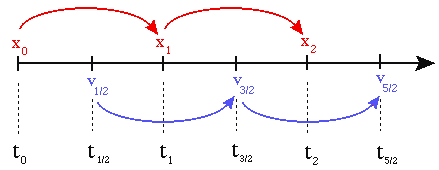
Notice that instead of using dt, we're using dt/2. i.e, we're updating the velocity at a half time-step. The reason for this is to implement leapfrog integration. The leapfrog method solves equations of motion with a second order accuracy (which is why it is preferred over the commonly used Euler's integration), by calculating velocity and position at staggered time points.
In our loop, first, the velocity is calculated at a half time-step, dt/2, followed by the position calculated at a full time-step dt, i.e, x and v are calculated such that they 'leapfrog' over each other. This makes our calculations more precise, although a bit slower.
…and now you have a simplified n-body simulation! By tweaking the initial settings such as velocity, position, and mass, you can observe how even small changes can result in vastly different outcomes, demonstrating the chaotic behavior we discussed earlier.
The full program can be accessed at :
https://github.com/fa22991/n-body-simulation-VPython/
Thank you for making it to the end!