How to detect exoplanets using the transit method

Exoplanets are planetary systems that lie far, far outside our own solar system. The problem with them being so far away is that we can’t visit them or see them directly with most telescopes. So then, how have astronomers detected over 6,000 of these planets orbiting distant stars already? The answer lies in analyzing data collected from telescopes and spacecrafts to find information that directly or indirectly confirms their existence.

One of the newer, and more efficient ways to do this is via the Transit method. In this article, I’ll go over how the Transit method works, and one of the best algorithms used to filter true transits from raw data- the Box Least Squares algorithm!

The Transit Method

This technique involves watching the brightness of stars over time and looking for the small dips caused when an orbiting planet passes in front of its host star, blocking some of its light.

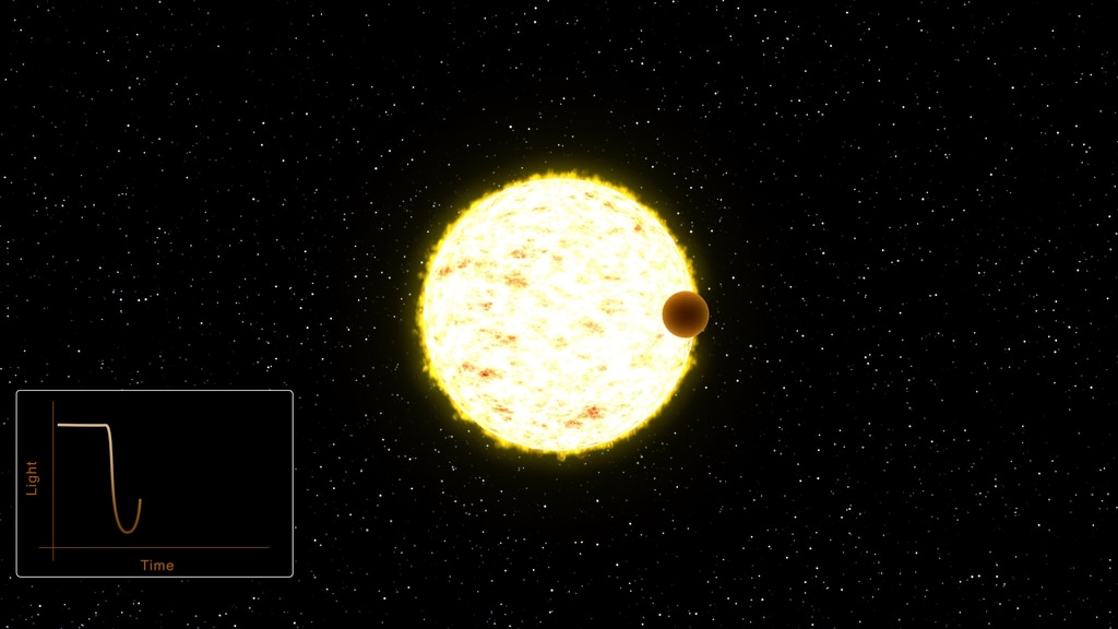
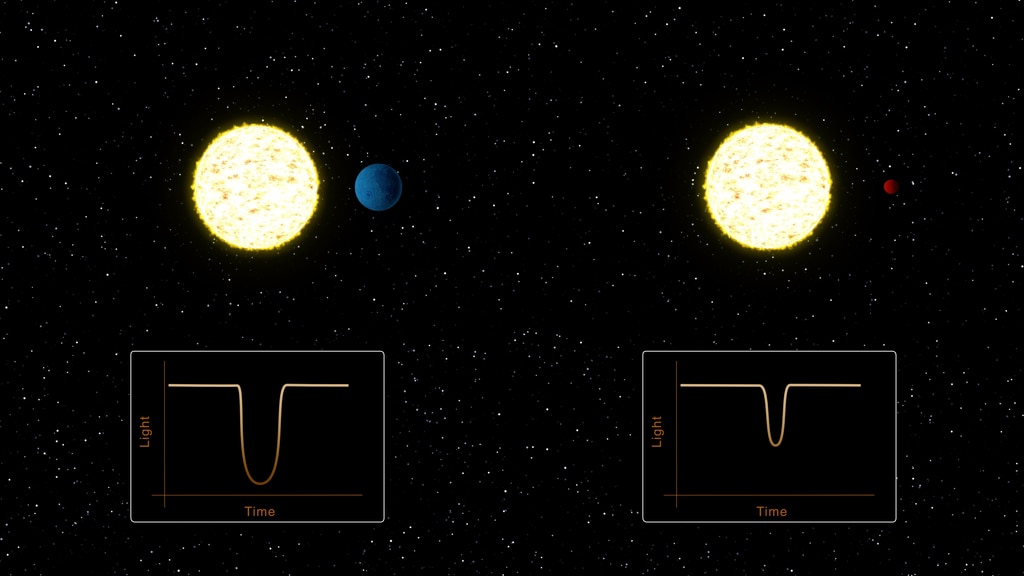
The transit produces a characteristic light curve (a graph of brightness versus time) with a slight, periodic dip in intensity caused by the orbiting exoplanet each time it blocks the part of the star observed by the telescope. The depth and duration of these dips provide important information about the planet’s size and orbit. A deeper drop usually indicates a larger planet, while the distance between drops gives us the exoplanet's orbital period.

Furthermore, we can use Kepler's third law of planetary motion to determine the distance of the exoplanet from its star. This information could give an idea as to whether the planet might possibly be in its host star's habitable zone (regions where the physical conditions may be just right for liquid water!).

Astronomers gather this data from space telescopes like NASA’s Kepler and TESS missions, which collect vast amounts of light intensity measurements over months and years. The raw data can be noisy due to instrumental effects or stellar activity, which is where computational methods help filter out true transits.

Box Least Squares (BLS)

One popular technique to do this is the Box Least Squares (BLS) algorithm. It works by dividing the light curve into equal sections, and phase-folding them (folding them on top of each other to fit within a mathematically determined period) to fit a simple box-shaped model. It tries many different possible values for this orbital period until finding one that results in the signals (dips in brightness) aligning.

Implementing BLS using Astropy and Matplotlib

Now that we know how this algorithm works, we can move on to analyzing some data ourselves! For this article, I’m using Kepler & TESS Exoplanet Data from Kaggle that contains information about confirmed exoplanets (since I’ll need a transit event to actually occur for me to demonstrate BLS). I’m not going to be plotting raw telescope data, rather, using these known planetary periods and radii I’ll simulate how a star's brightness would look if these planets were passing in front of it.

Let’s start by importing all the external libraries we’ll need,

import numpy as np
import matplotlib.pyplot as plt
import pandas as pd
from astropy.timeseries import BoxLeastSquares

Then, we can write a function to simulate a light curve from the planet’s data as shown below.

def simulate_lightcurve(period, radius, n_points=1000):
    time = np.linspace(0, max(period)*3, n_points)
    flux = np.ones_like(time)

    for p, r in zip(period, radius):
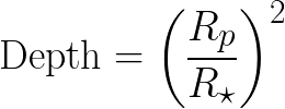
        depth = (r * 0.009158)** 2
        duration = 0.1 * p
        phase = (time % p) / p
        in_transit = (phase < duration/p)
        flux[in_transit] -= depth

    return time, flux

This function generates an array time[] that covers three orbits of the planet with the longest period and initializes the normalized brightness (flux) as 1. Then, for each planet it calculates the expected transit depth using the formula-

phase = (time%p) / p folds the continuous timeline into repeating cycles between 0 and the period p. in_transit is a Boolean array that contains all time points that fall within the transit window. We then subtract the depth of the transit from the flux array at times when the light curve is in the transit event. Finally, we return the synthetic combined light curve representing all planets’ transits.

We can then write another function called bls_implementation() that extracts the period and radius from the Kaggle dataset and calls simulate_lightcurve() using them as parameters.

def bls_implementation(csv_path, max_planets=5):
    # Load kaggle data
    df = pd.read_csv(csv_path, comment='#')

    # Extract planets with valid orbital period and radius (Earth radii)
    planets = df[['pl_orbper', 'pl_rade']].dropna()

    # Filter realistic values
    mask = (planets['pl_orbper'] > 0) & (planets['pl_rade'] > 0)
    planets = planets[mask]

    # Limit to first 'max_planets' for simulation clarity
    sample = planets.head(max_planets)
    periods = sample['pl_orbper'].values
    radii = sample['pl_rade'].values

    # Simulate combined light curve for selected planets
    time, flux = simulate_lightcurve(periods, radii, n_points=5000)

Here, pl_orbper and pl_rade are column names in the csv file that correspond to a planet’s orbital period and radius.

Now for the BLS implementation, we can use Astropy’s BoxLeastSquares function as such :

    flux = flux / np.nanmedian(flux)

    # Compute BLS periodogram
    bls = BoxLeastSquares(time, flux)
    periods_grid = np.linspace(0.5, 1.5*max(periods), 20000)
    results = bls.power(periods_grid, 0.1)

    # Find best period peak
    best_idx = np.argmax(results.power)
    best_period = periods_grid[best_idx]
    best_power = results.power[best_idx]

We first normalizes the brightness data, so all the flux values are centered around 1 by dividing by their median. This makes it easier to detect subtle dips caused by planetary transits. Then, we apply the Box Least Squares (BLS) algorithm to the normalized light curve over a range of possible orbital periods, searching for the best-fitting periodic box-shaped dip which represents the transit signal of a planet passing in front of its star. The code finds the period with the highest detection power, which is likely the planet’s orbital period.
We have orbital period data in our CSV file, allowing us to visualize the expected transit. However, real-world exoplanet hunters don't have this luxury. That's why they rely on algorithms like BLS, which provide highly accurate period values. We'll demonstrate this accuracy by plotting the light curve we simulated (based on real exoplanet periods and radii) alongside the BLS model's prediction below.

    # Plot combined light curve & BLS periodogram
    best_t0 = results.transit_time[best_idx]
    best_dur = results.duration[best_idx]
    model = bls.model(time, best_period, best_dur, best_t0)

    fig, (ax1, ax2) = plt.subplots(2,1, figsize=(10,7), gridspec_kw={'height_ratios':[2,1]})
    ax1.plot(time, flux, 'k-', markersize=2, alpha=0.6, label='Simulated Flux')
    ax1.plot(time, model, 'r-', lw=1.5, label='BLS Transit Model')
    ax1.axvspan(best_t0 - 0.5*best_dur, best_t0 + 0.5*best_dur, color='r', alpha=0.1)
    ax1.set_xlabel('Time (days)')
    ax1.set_ylabel('Normalized Flux')
    ax1.set_title('Simulated Exoplanet Transit Light Curve')
    ax1.legend()

    ax2.plot(periods_grid, results.power, 'k-')
    ax2.axvline(best_period, color='purple', linestyle='--', label=f'Best Period = {best_period:.5f} d')
    ax2.set_xlabel('Period (days)')
    ax2.set_ylabel('BLS Power')
    ax2.legend()

    plt.tight_layout()
    plt.show()

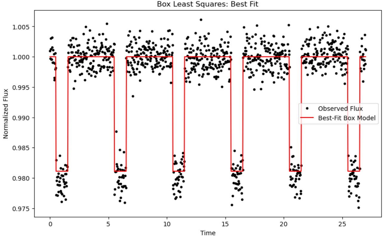
Calling bls_implementation() on the Kaggle data should result in a plot that looks something like this :

From the first plot, we see that the time intervals for the simulated curve and the BLS model overlap almost entirely! However, the depth of the transit is significantly lower in the model. One possible reason for this is that because the BLS algorithm fits a simplified "box-shaped" model and works with imperfect data, it often estimates a shallower (less deep) transit depth than the idealized simulated transit that perfectly uses known planet size and orbit like the one in our confirmed exoplanets catalog. Still, we see that BLS matches the intervals between transits almost exactly, confirming the orbital period and reliably pinpointing when each transit occurs!

Conclusion

So, what does all this mean? Basically, by using real exoplanet data to simulate how these planets would block their stars, and then applying the BLS algorithm to detect those dips in light intensity, we can get an idea of how transit detection actually works. The simulation gives us a clear, ‘ideal' picture of the transits, while BLS finds those signals in messier data that has some noise (like the data you’d get from a telescope). Even though the depths of the transits might not perfectly match, BLS discerns the timing of their occurrence almost exactly, which is what really matters when confirming and discovering planets.

Thank you for reading! All the code can be found below :

https://github.com/fa22991/bls_algorithm_for_exoplanet_detection